Building a factor-tilted equity portfolio: Our experience
Zsolt writes about how building a custom factor-tilted equity portfolio allowed Titanium Birch to move beyond ETF combinations and systematically translate our investment views into disciplined, data-driven portfolio weights.
The content in this post should not be taken as investment advice and does not constitute any offer or solicitation offering or recommending any investment product.
Why we went custom on equities
In earlier versions of our portfolio, our equity exposure initially came through well-known, off-the-shelf solutions in the form of popular ETFs. These products are liquid, transparent, and easy to use, and they served us well for quite some time. Over time, however, we realized that implementing our desired exposures using standard ETFs was not straightforward. Because ETF holdings often overlap, combining several funds can easily lead to unintended concentrations — for example, excessive exposure to certain companies or sectors — which could breach our internal risk limits.
At the same time, we had certain views we wanted to express in our portfolio allocation — such as reducing the weight of stocks that appear overpriced — but without becoming active stock pickers. Instead, we were looking for a way to translate these views into systematic portfolio decisions.
We evaluated several third-party solutions and spoke with a number of vendors. Ultimately, however, we found that our particular requirements were easier to implement with a custom approach.
This led us to explore implementing factor tilts directly at the stock level rather than through ETF combinations. Factor tilting offers a way to start from a diversified market portfolio while introducing disciplined adjustments based on measurable characteristics.
Finally, on a more practical note, our team has reasonably good data skills and, as a learning project, we wanted to tinker with the data at hand so that we can learn and appreciate the complexities of the topic.
Quick primer: What is factor tilting?
For decades, academic research has sought to understand and decompose the drivers of equity returns. Rather than searching for a “secret sauce,” researchers have tried to identify systematic sources of risk and return that persist over time.
Early models such as the Capital Asset Pricing Model (CAPM) suggested that expected returns are primarily driven by exposure to market risk. Later research showed that additional characteristics, known as factors, also help explain differences in returns. In the early 1990s, Eugene Fama and Kenneth French formalized this idea in their three-factor model, adding size and value to market beta. Subsequent research expanded the framework further to include factors such as profitability, investment, and momentum.
In Your Complete Guide to Factor-Based Investing, Andrew Berkin and Larry Swedroe emphasize that not every documented anomaly deserves to be treated as a reliable factor. Academic literature contains hundreds of proposed factors, often referred to as the “factor zoo.” To separate robust drivers from statistical noise, they propose a practical framework: a factor should be intuitive, persistent across time and regions, robust to alternative definitions, and investable after costs.
Based on these criteria, a small set of factors has been widely studied and implemented:
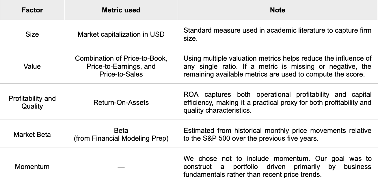
Market beta – exposure to overall market risk (as captured by CAPM)
Size – smaller companies have historically delivered higher expected returns than larger ones
Value – companies trading at lower valuations relative to fundamentals have tended to outperform more expensive peers
Momentum – stocks with stronger recent performance have often continued to perform well in the near term
Profitability / Quality – firms with stronger profitability metrics have exhibited more attractive return characteristics than weaker firms
Factor tilting builds on this foundation. Rather than holding each stock strictly in proportion to its market weight, a portfolio can modestly increase exposure to these characteristics while maintaining broad diversification.
From idea to portfolio: Our approach
To translate the factor ideas discussed above into an investable portfolio, we designed a simple workflow that maps the key inputs and calculations required in our process.
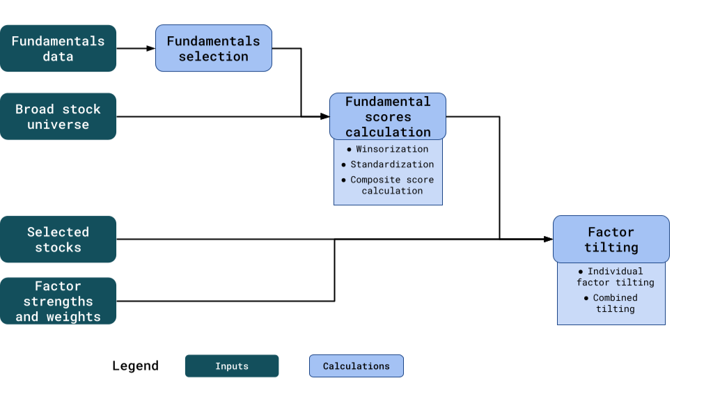
The diagram illustrates the steps involved in transforming raw financial data into factor-tilted portfolio weights. At a high level, the process begins with gathering and selecting fundamental data, which is then transformed into standardized factor scores that can be used to tilt portfolio weights.
Fundamentals data
We obtain company fundamentals from Financial Modeling Prep, which we selected for its broad global coverage, reasonable data quality, and straightforward API endpoints.
Broad stock universe
This universe provides the reference distribution for our financial metrics — allowing us to determine what constitutes typical, extreme, or outlier values. In our case we used a broad market universe similar in scope to the holdings of the Vanguard Total Market ETF (VT).
Fundamentals selection
For each factor, we selected a small set of intuitive and widely used financial metrics to capture the underlying economic characteristic:
Fundamental scores calculation
The selected financial metrics need to be transformed into standardized scores that are comparable across companies. We apply the following data processing steps (excluding the Size factor, which is used directly):
Winsorization
Financial datasets often contain extreme outliers that can distort calculations. To mitigate this, we winsorize each metric by capping extreme values at predefined thresholds. This helps prevent a small number of unusual observations from dominating the factor scores.
Standardization
The financial metrics used in the model are expressed in different units and scales. To make them comparable, we standardize each metric using a z-score transformation:
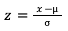
where 𝑥 is the observed value, 𝜇 is the mean across the universe, and 𝜎 is the standard deviation. This transformation expresses each company’s metric relative to the distribution of the broader universe.
Combined factor scores
Some factors rely on multiple metrics. In our case, the Value factor combines several valuation ratios (Price-to-Book, Price-to-Earnings, and Price-to-Sales). The standardized scores of the available metrics are averaged to produce a single factor score.
Composite score transformation
Finally, the raw z-scores are transformed into composite scores using the following rule:
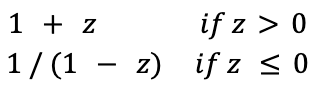
This transformation preserves the relative ordering of companies but changes the shape of the distribution. Companies with stronger financial characteristics (higher z-scores) receive proportionally larger composite scores, while weaker companies are compressed toward lower values.
The effect of this transformation is illustrated below.
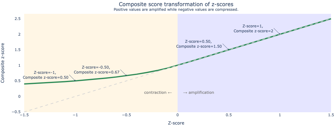
By applying this transformation, companies with stronger fundamentals become more clearly differentiated in the scoring system, which allows the subsequent factor tilting step to allocate weights more meaningfully.
Factor tilting
Once the fundamental scores have been calculated, the next step is to translate them into portfolio weights through factor tilting.
We begin with a predefined set of investable stocks — for example the constituents of the S&P 500 — together with their baseline weights. In most cases, these baseline weights correspond to the market-capitalization weights of the stocks within the index.
The precalculated fundamental scores are then merged with this stock universe, allowing us to systematically adjust the baseline weights based on the desired factor exposures.
Our factor tilting process consists of two stages:
Individual factor tilts – adjusting weights based on each factor separately (e.g. size, value, or profitability).
Combined factor tilts – aggregating the individual tilts into a single adjustment applied to the portfolio weights.
The following sections describe these two steps in more detail.
Individual factor tilts
To apply factor tilts, we introduce a tilt strength parameter that controls how strongly a factor influences the portfolio weights. A strength of 0 corresponds to no tilt (the original market weights are preserved), while larger values increase the impact of the factor.
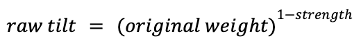
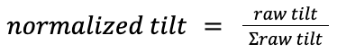
We calculate raw tilts using the following formulas.
Size:
This transformation progressively flattens the distribution of market-cap weights as the tilt strength increases.
All other factors:

Here the factor score acts as a multiplier on the baseline portfolio weight, increasing the weight of companies with stronger factor characteristics.
After calculating the raw tilts, we normalize them so that the weights sum to one:
Example: Size tilting
To illustrate the impact of the strength parameter, consider a portfolio of 50 companies with market-cap–weighted baseline weights.
The chart below shows how the portfolio weights change under different tilt strengths.
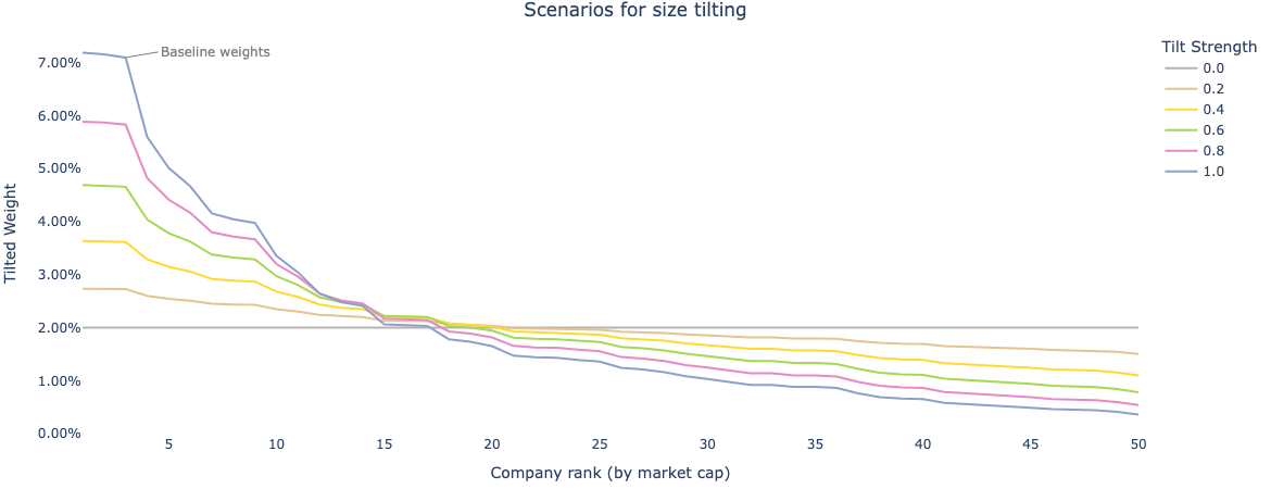
When the strength parameter is 0, the original market-cap weights are preserved. As the strength increases, the weight distribution gradually flattens. At a strength of 1, the portfolio becomes equally weighted, meaning each company receives the same weight (in this example, 100% / 50 = 2%).
In practice, we typically restrict the strength parameter to values between 0 and 1. While larger values are mathematically possible — and could be used to produce extremely strong value or profitability tilts — they can significantly distort the original market-cap structure of the portfolio. In early experiments we found that such extreme tilts introduced risks that felt disproportionate to the intended factor exposure.
Combined factor tilts
Once the individual factor tilts have been calculated, the next step is to combine them into a single portfolio adjustment. We do this by taking a weighted average of the individual factor tilts, using manually assigned weights for each factor.
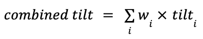
where wᵢ represents the weight assigned to factor i.
Example
Consider a company from the S&P 500 with the following weights and individual factor tilts:
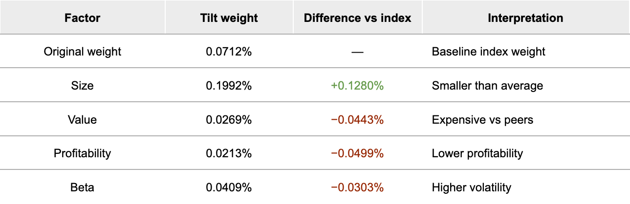
Suppose we decide to place less emphasis on size and more emphasis on the fundamental factors. We might assign the following weights to the factor tilts:
Size: 15%
Value: 25%
Profitability: 45%
Beta: 15%
Applying these weights produces a combined tilt weight of 0.0523% for this company. Compared with the original index weight of 0.0712%, this implies that the tilted portfolio would allocate roughly 26% less capital to this company than the index would.
Portfolio impact of the tilting framework
To illustrate the overall effect of the tilting process, we applied the factor weights from the example above to the S&P 500 constituents and compared the resulting portfolio characteristics with those of the original index.
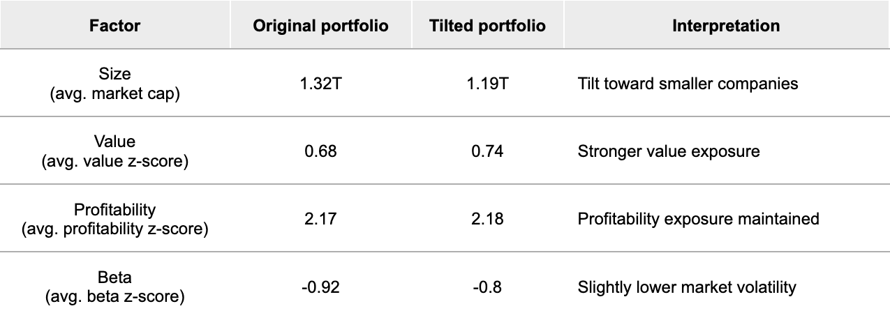
With these settings, the portfolio achieves a modest increase in value exposure, shifts toward smaller companies, and slightly reduces market beta, while maintaining strong profitability characteristics.
The example above also highlights an important design choice in our framework: how the weights assigned to each factor tilt are determined. In the current version of our framework, these weights are set manually. We choose them to ensure that the resulting portfolio remains within our risk limits while also reflecting our views on which factors are likely to perform well.
In the broader factor-investing literature, these weights are often determined using portfolio optimization techniques, where the objective is to maximize expected return subject to risk constraints. While our current approach keeps the process transparent and easy to interpret, exploring optimization-based approaches is something we may consider in future iterations.
Results and learnings
Overall, as a team, we are quite pleased with the outcome of this first iteration of the project.
First, we successfully constructed a portfolio that remains within our predefined risk limits while still allowing us to apply factor tilts. Achieving this balance was an important objective from the start.
Second, the framework gives us a practical way to express our views on different factors and their relative importance. By adjusting the factor parameters, the tool recalculates the portfolio weights automatically, which allows us to compare different portfolio versions and iterate quickly.
At the same time, the project revealed several areas where the model can be improved.
One challenge is the number of parameters involved. Each factor currently has both a tilt strength and a factor weight, which creates many possible combinations that can satisfy the portfolio constraints. In practice, manually coordinating these parameters proved difficult. As a pragmatic first step, we chose to set all tilt strengths to 1 and focus on fine-tuning the factor weights instead.
We also relied on a relatively standard set of financial metrics to represent the factors. While these worked well as a starting point, we see two natural directions for further research:
exploring whether alternative financial metrics could better capture the existing factors
investigating additional factors that may be particularly relevant in certain markets or environments
Finally, we are also mindful that the effectiveness of certain factors can vary across time periods. Both the size and value factors have experienced extended periods of weak performance in recent years, as discussed by Professor Damodaran. We plan to examine these patterns more closely and reassess how strongly these factors should influence our portfolio construction going forward. This framework is still evolving, and we expect it will continue to change as we learn more.
If projects like this resonate with you, we are currently hiring a decision systems engineer who enjoys working with data to build tools for systematic investing.
Disclaimer
The content in this post should not be taken as investment advice and does not constitute any offer or solicitation offering or recommending any investment product.
The constituents of the Vanguard Total World ETF and S&P 500 are used purely as illustrative universes for the example and do not imply any affiliation with or endorsement by S&P Dow Jones Indices or Vanguard.